

From: http://cis.legacy.ics.tkk.fi/aapo/papers/IJCNN99_tutorialweb/node26.html
Another useful preprocessing strategy in ICA is to first whiten the observed variables. This means that before the application of the ICA algorithm (and after centering), we transform the observed vector ![]() linearly so that we obtain a new vector
linearly so that we obtain a new vector ![]() which is white, i.e. its components are uncorrelated and their variances equal unity. In other words, the covariance matrix of
which is white, i.e. its components are uncorrelated and their variances equal unity. In other words, the covariance matrix of ![]() equals the identity matrix:
equals the identity matrix:
| (30) |
The whitening transformation is always possible. One popular method for whitening is to use the eigen-value decomposition (EVD) of the covariance matrix![]() , where
, where ![]() is the orthogonal matrix of eigenvectors of
is the orthogonal matrix of eigenvectors of ![]() and
and ![]() is the diagonal matrix of its eigenvalues,
is the diagonal matrix of its eigenvalues, ![]() . Note that
. Note that ![]() can be estimated in a standard way from the available sample
can be estimated in a standard way from the available sample ![]() . Whitening can now be done by
. Whitening can now be done by
where the matrix
Whitening transforms the mixing matrix into a new one, ![]() . We have from (4) and (34):
. We have from (4) and (34):
| (32) |
The utility of whitening resides in the fact that the new mixing matrix
| (33) |
Here we see that whitening reduces the number of parameters to be estimated. Instead of having to estimate the n2 parameters that are the elements of the original matrix
It may also be quite useful to reduce the dimension of the data at the same time as we do the whitening. Then we look at the eigenvalues dj of ![]() and discard those that are too small, as is often done in the statistical technique of principal component analysis. This has often the effect of reducing noise. Moreover, dimension reduction prevents overlearning, which can sometimes be observed in ICA [26].
and discard those that are too small, as is often done in the statistical technique of principal component analysis. This has often the effect of reducing noise. Moreover, dimension reduction prevents overlearning, which can sometimes be observed in ICA [26].
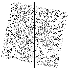
A graphical illustration of the effect of whitening can be seen in Figure 10, in which the data in Figure 6 has been whitened. The square defining the distribution is now clearly a rotated version of the original square in Figure 5. All that is left is the estimation of a single angle that gives the rotation.
In the rest of this tutorial, we assume that the data has been preprocessed by centering and whitening. For simplicity of notation, we denote the preprocessed data just by ![]() , and the transformed mixing matrix by
, and the transformed mixing matrix by ![]() , omitting the tildes.
, omitting the tildes.
No comments:
Post a Comment